Demo and applications

This website will present (partly preliminary) results from applying several machine learning and mathematics techniques to different atmospheric topics.

Creation of semi-empirical autoxidation chemistry schemes

In this project we aiming to create lumped reaction schemes for highly complex chemical systems like the oxydation of volatile organic compounds (VOC). The method is characterised by an iterative process of scheme creation, empiric rate coefficient assignment, stochastic testing, and AI-driven network analysis to highlight missing dependencies in the chemistry schemes. As a result, the degree of lumping is automatically adjusted to the experimentally reported complexity of a VOC system.

Toy-case approach

We have created a ‘toy’ scheme with one fictional precursor VOC to test and demonstrate all computational approaches
(press here to see the full toy-case chemistry scheme).

This chemistry scheme aims to reflect the complex interactions and main reaction pathways in the autoxidation of carbon-centred radicals. The precursor chemical species is a fictional VOC called TOY. In this scheme, autoxidation reactions (see “Autoxidation: RO2 -> H-shift + O2 addition -> RO2 ” in the scheme) are competing bimolecular reactions (RO₂ + NO/HO₂/RO₂) leading to the formation of stable, closed shell species (RO₂ + NO: T_O*_NO3; RO₂ + HO₂: T_O*_OOH; and RO₂ + RO₂: T_O*_2OH, T_O*_O and TO*_TO*; where * represents integer numbers). Additionally, there are reaction branches that form highly reactive alkoxy radicals (T_RO_O*). These can rapidly (rate: KDEC = 10⁶ s-1) undergo autoxidation form peroxy radicals (T_RO2_O*).

To investigate the toy-chemistry, the following states of the chemistry are intended in order to determine multi-experiment based, realistic rate coefficients (see Pichelstorfer et al., 2024 , section 3.3 for more details):

1) Low NO, HO₂ and VOC turnover (i.e., the reactions consuming the TOY-VOC) will maximize the RO₂ autoxidation reaction.
2) Strong increase in NO, HO₂ or VOC-turnover will shift the system towards closed shell formation (nitrates/hydroperoxides and dimers)
3) Medium increase in NO, HO₂ or VOC-turnover will highlight autoxidation via the alkoxy pathway (T_RO_O* → RO₂)

To investigate the effects, branching ratios of the reactions may be varied, e.g.: RO2 + NO → a) RONO2 and b) alkoxy may be either shifted to higher nitrate formation: increase channel a), or to see higher alkoxy radical formation: increase path b). Similarly, the branching in the H-shift reaction forming a peroxy radical (i.e., the RO2) and its competing reaction pathway to form a closed shell species (Tuni_O*_O) may be changed to either promote autoxidation or to limit it by the (almost) unimolecular termination pathway.

The formation of adducts, which typically are very low-volatility species, is important for the early growth of nano-clusters. It can be enhanced by keeping the NO and HO₂ low while increasing the VOC-turnover. In case they don’t form sufficiently, the competing reaction pathways can be tuned down (i.e., the reactions with the sum of RO₂ which are indicated by the term “RO2” in the rate coefficient).

AutoCONSTRAINT work:

Pichelstorfer, L., O’Meara, S. P., and McFiggans, G. B.: Theory informed, experiment based, constraint on the rate of autoxidation chemistry – An analytical approach, Aerosol Research Discuss. [preprint], https://doi.org/10.5194/ar-2024-40, in review, 2024.

Applying autoCONSTRAINTS

To infer rate coefficients for the autoREACTIONS-generated autoxidation scheme (see table xx), we applied the same steps as outlined in a recent work introducing the autoCONSTRAINTS method (Pichelstorfer et al., 2024):

1) we considered “experimental data” generated by means of modelling applying the PyCHAM box-model;
2) model data complementing the experimental inputs was generated the same way to quantify parameters typically not observed experimentally (concentrations of NO, HO₂ and the sum of RO₂);
3) in a next step a change-rate equation for each mass peak is set up (i.e. equation 2 in Pichelstorfer et al., 2024)
4) A guess on the relative magnitude of the reaction rate coefficients describing the production of the same atomic mass peak allows to solve the equation set up in step 3. Reaction rate coefficients found and their precision (with respect to set rate coefficients of the autoREACTIONS generated autoxidation scheme) are depicted by Figures 1 to 5.

Figure 1: Peroxy radicals (names given by the abscissa) react at a rate (denoted on the lower ordinate) to form RO₂. The precision of rate coefficient recovery from the (simulated) mass spectrum is shown on the upper ordinate (recovered over set rate coefficient).

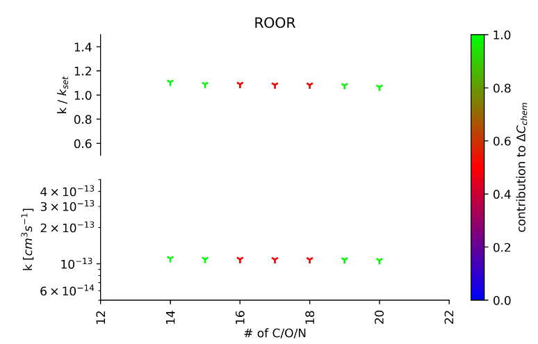
Figure 2: The abscissa shows peroxy radicals (denoted by their number of carbon + oxygen + nitrogen atoms) reacting at the rate coefficient k (lower ordinate) to form ROOR species. The precision of rate coefficient recovery from the (simulated) mass spectrum is shown on the upper ordinate (recovered over set rate coefficient). The colour code denotes the calculated contribution of the reaction to the change (by means of chemical reactions) in CIMS mass peak concentration.

Figure 3: RO₂ radicals (names given by the abscissa) react at a rate (denoted on the lower ordinate) to form RONO2 (downward facing triangle), alkyl species (upward facing triangles), fragmentation species (plus) and alkoxy radicals (crosses). A circle shows the sum of the individual reaction channel’s rates. The precision of rate coefficient recovery from the (simulated) mass spectrum is shown on the upper ordinate. The colour code denotes the calculated contribution of the reaction to the change (by means of chemical reactions) in CIMS mass peak concentration.

Figure 4: Peroxy radicals (names given by the abscissa) react at a rate (denoted on the lower ordinate) to form ROH (downward facing triangle), alkyl species (upward facing triangle) and alkoxy radicals (crosses). A circle shows the sum of the individual reaction channel’s rates. The precision of rate coefficient recovery from the (simulated) mass spectrum is shown on the upper ordinate (recovered over set rate coefficient). The colour code denotes the calculated contribution of the reaction to the change (by means of chemical reactions) in CIMS mass peak concentration.

Figure 5: peroxy radicals (names given by the abscissa) react at a rate (denoted on the ordinate lower) to form ROOH (downward facing triangle) and alkoxy radicals (crosses). A circle shows the sum of the individual reaction channel’s rates. The precision of rate coefficient recovery from the (simulated) mass spectrum is shown on the upper ordinate (recovered over set rate coefficient). The colour code denotes the calculated contribution of the reaction to the change (by means of chemical reactions) in CIMS mass peak concentration.

Uncertainty quantification of the rate coefficients with MCMC

The reaction rate constants should be calibrated using measured mass spectra. However, the situation is ill-posed: the reaction schemes consist of a high number of reactions, while the experimental data for each autoxidation module is limited to a handful of mass spectra with limited measurement accuracy. We demonstrate here the impact of measurement uncertainty in the toy case. We assume ideal data: all concentrations are measured at several time points, and a small relative noise of 5 per cent is added. Adaptive MCMC methods (Haario H., et al., Stat. Comput., 16,339-354, 2006; Wang, S., et al., Environ. Sci. Technol., 51, 8442−8449, 2017) are then used to find ‘all’ reaction rate values that agree with the data within the measurement accuracy.

Figures 6, 7, and 8 show the histograms of the sampled parameter values in scaled units. The system is sensitive to several reaction rates: the parameters remain close to the default value 1. However, some parameters have much larger histogram ranges, even close to a uniform distribution between the minimum and maximum bounds set. This means that the system is more insensitive to changing those reaction rates.

Figure 9 verifies the approach: we simulate the system using all the different parameter combinations found by the MCMC sampling and construct the histograms of the concentration values at the final steady-state observation point. We can see how, in scaled units again, the concentration values are tightly fitted around the correct synthetic data values at roughly 5 per cent accuracy.

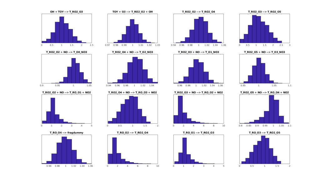
Figure 6: Histograms of the sampled parameter values in scaled units. (Reactions 0-15).

Figure 7: Histograms of the sampled parameter values in scaled units (Reactions 15-31).

Figure 8: Histograms of the sampled parameter values in scaled units (Reactions 32-48).

Figure 9: Histograms of the concentration values at the final steady-state observation point.

Graphical Neural Network for chemical reaction rate estimation

The chemical schemes describing autoxidation are detailed; however, they are still lumped. As a result, a scheme may not serve to explain all chemical regimes experimentally investigated. To overcome this, GNN is set up to highlight dependencies (e.g., reaction pathways) not covered so far. Findings will be converted to chemical reactions and considered in a new, autoREACTIONS-created chemical scheme. The complex chemical system can be represented as a chemical graph with nodes and edges. GNN efficiently processes chemical graphs to learn the intricate connections and adjust weights accordingly to capture important relationships. We will utilise the knowledge of the obtained rate coefficients to initialise GNN’s parameters and optimise it for exploring novel associations between newly generated chemical components and others present in the system. Moreover, GNN can include meteorological variables (temperature, humidity, etc.) to learn about changes in chemistry paths in different physical environments.

Figure 10: Pipeline of using the neural network for chemical reaction rate estimation

Figure 11: Reaction rate estimation between ground truth and our estimation for the toy-case

Neural Emulator for chemical concentration prediction

Modelling atmospheric chemistry is complex and computationally intense. Given the recent success of Deep neural networks in digital signal processing, we propose a Neural Network Emulator for fast chemical concentration modelling (Figure 1). We consider atmospheric chemistry as a time-dependent Ordinary Differential Equation. To extract the hidden correlations between initial states and future time evolution, we propose ChemNNE, an Attention based Neural Network Emulator (NNE) that can model atmospheric chemistry as a neural ODE process. We implement sinusoidal time embedding to efficiently capture temporal patterns in chemical concentration changes to represent periodic tendencies over time.
Additionally, we leverage the Fourier neural operator to model the ODE process, enhancing computational efficiency and facilitating the learning of complex dynamical behaviour. We introduce three physics-informed loss functions, targeting conservation laws and reaction rate constraints, to guide the training optimisation process. To evaluate our model, we introduce a unique, large-scale chemical dataset designed for neural network training and validation, which can serve as a benchmark for future studies. The extensive experiments show that our approach achieves state-of-the-art performance in modelling accuracy and computational speed (Figure 2).

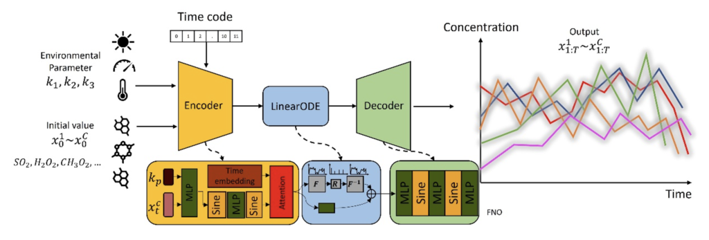
Figure 1: The proposed ChemNNE for chemical concentration prediction. It takes the environmental parameters and initial chemical concentration to predict the future chemical reaction process.

Figure 2: Visualization of the time evolution of chemistry. In (a), (b), and (c), we show the ground truth as red lines and the predictions with different colours. We pick four different chemical compounds for comparison and enlarge the region in red boxes to highlight the prediction errors.

Deep Spatio-Temporal Neural Network for Air Quality Reanalysis

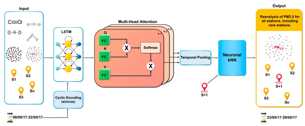
Air quality prediction is key to mitigating health impacts and guiding decisions, yet existing models tend to focus on temporal trends while overlooking spatial generalization. We propose AQ-Net, a spatiotemporal reanalysis model for both observed and unobserved stations in the near future. AQ-Net utilizes the LSTM and multi-head attention for the temporal regression. We also propose a cyclic encoding technique to ensure continuous time representation. To learn fine-grained spatial air quality estimation, we incorporate AQ-Net with the neural kNN to explore feature-based interpolation, such that we can fill the spatial gaps given coarse observation stations. To demonstrate the efficiency of our model for spatiotemporal reanalysis, we use data from 2013–2017 collected in northern China for PM 2 . 5 analysis. Extensive experiments show that AQ-Net excels in air quality reanalysis, highlighting the potential of hybrid spatio-temporal models to better capture environmental dynamics—especially in urban areas where both spatial and temporal variability are critical.

The code can be found at AQ-Net.

Our model predicts PM2.5 by combining temporal and spatial dependencies. AQ-Net comprises three core components: an LSTM-MHA module, combining LSTM and multi-head attention for temporal feature extraction, a neural kNN module for spatial interpolation, and a Cyclic Encoding (CE) layer for time embedding. We use hourly measurements of PM2.5, PM10, CO, NO2, SO2, and O3 from monitoring stations, and estimate PM2.5 for the coming hours and days. The LSTM captures long-range pollutant fluctuations, while multi-head attention highlights critical time steps. A temporal pooling step condenses the latent sequence into a single feature vector, which the neural kNN module uses for spatial interpolation at unobserved stations based on their nearest neighbors. This integrated architecture generates 168-hour (7-day) PM2.5 estimation for both observed and unobserved locations, leveraging key temporal patterns and spatial relationships.

To illustrate the efficiency of our proposed AQ-Net on the large-scale dataset, we show spatiotemporal reanalysis in the entire northern China. As shown in Figure 3, utilizing the proposed neural kNN, we are able to estimate the complete spatial interpolation, capturing both observed and unobserved areas. Notably, pollution hotspots around northern and central Beijing are consistent with known urban emission sources. These results highlight the model’s ability to generalize beyond monitored stations, which is crucial for accurate city-wide air quality assessments.

About

Contact Us

contact@amc-lahti.fi

Location

LAHDEN YLIOPISTOKAMPUS Niemen kampus Niemenkatu 73 (B-osa) 15140 Lahti